INTRODUCTION
There have been a wide variety of pitching biomechanics studies performed over the past 20+ years using optical motion tracking, electromagnetic, and more recently inertial sensor systems. The papers from Whiteley 2007 and Chu 2012 provide extensive reference lists for a summary of pitching biomechanics studies using optical and electromagnetic systems for the interested reader. The purpose of this post is to compare the published values for pitching arm side (PAS) kinematics from a few important pitching biomechanics studies. I will compare research studies from Fleisig et al., 1995, Aguinaldo et al., 2007, and Chu 2012 that all used optical motion capture systems but with different marker protocols. I will also compare results from Lapinski et al., 2009 and Lapinski 2013 that used an inertial sensor system with multiple nodes for analyzing pitching and hitting biomechanics. Specifically, this post will examine the effect that different measurement systems and kinematic calculation methodologies have on reported values for humeral external rotation, internal rotational angular velocity, and angular acceleration measurements. In the ASMI limitations page, I provided details on why ASMI methodologies can only provide qualitative kinematic values for these shoulder rotational values.
Optical motion capture data is known to provide accurate 3D positional data. Orientation data calculated from the 3D positional data is also considered to be relatively accurate. Where optical motion capture data can be limited in accuracy is when the positional data is differentiated once for velocity data and twice for acceleration data. Filtering techniques typically not only filter the data to remove noise from the marker data, but they tend to smooth the velocity and acceleration data as well. The question in high-speed dynamic sports movements is if the filtering/smoothing technique attenuates these rate changes too much or eliminates fidelity from the kinematic curves by removing accelerations and decelerations that actually exist in the movement pattern. Inertial sensors directly measure angular velocities and linear accelerations and as such provide more direct measurements for these parameters. Calculating positional and orientation data from these sensors is a much more difficult task and is not as accurate as directly measuring 3D positional data with an optical motion capture system.
The biggest question to sports scientists is what system provides the best results for high-speed movement and loading pattern analysis. The choice of which system technology to use has only really become a decision in the last decade or so, and commercially available systems with more than one inertial sensor are still not really available to the general public. However, that is changing very rapidly and commercially available inertial sensor systems will become more available in the next few years. This post will critically review the previously mentioned papers for their ability to accurately measure the underlying skeletal kinematics for the shoulder kinematic values during the very dynamic pitching motion. The results from this evaluation will help determine which system is best for:
- Player Profiling: angular velocity of high-speed sports motions has proven to be a very powerful tool for characterizing athletes based on the resultant rotations of the end-effector segments in the kinematic chain. Accuracy in these measurements is imperative when analyzing single axis dynamic plots or plotting multi-axis angular velocity curves against one another.
- Angular acceleration: while angular velocities are good for profiling athletes, they are limited as they only provide how fast the bone is rotating; angular accelerations are better indicators for the rate of loading as they provide measurements for the acceleration and deceleration of the bones in the joint of interest. These values are more directly correlated to the rate of loading across joint soft tissues, which is very important for any detailed injury analysis.
- Forward dynamic simulations: physics-based dynamic simulations are a very powerful tool for orthopaedic and sports performance analyses. This modeling and simulation technique uses estimated joint torques to predict end-effector motions. This requires very accurate acceleration data in order for development of a model that can replicate input motion data with high correlation coefficients (> 0.95 for all model DOF). Once developed, these Virtual Product testing tools are extremely powerful.
SHOULDER KINEMATICS
The shoulder and shoulder girdle is the most complex joint of the human body as no other joint is tasked with the requisite combination of extreme mobility and dynamic stability. This joint is typically modeled as a ball-and-socket joint with 3 degrees of freedom (DOF). The glenohumeral (GH) joint is comprised of the humerus and scapula, and the coordinated movement between the two bones is crucial for athletic performance and maintaining health. Normal scapular kinematics are important for injury prevention as the scapula elevates the acromion to clear the subacromial space in overhead positions. Details on anatomical considerations and kinematic considerations of the shoulder complex are discussed elsewhere on this site, including details on scapular function and scapular dysfunction often found in pitchers. Being able to measure and evaluate scapulohumeral rhythm is critical if a sports scientist truly wants to quantitatively analyze performance and injury risks in elite level pitchers. Unfortunately, very few pitching biomechanics studies have included scapular kinematics in their measurement methodologies.

One of the most misunderstood requirements of an elite level pitcher is the dynamic scapular stability required for the extreme 3 DOF humeral range of motion (ROM) observed during the dynamic pitching motion. While trainers like Eric Cressey that specialize in the overhead throwing athlete understand and do a great job of explaining this, too many baseball personnel do not truly understand the importance of scapular kinematics and stability in the dynamic pitching motion. The scapula serves as a critical link in the kinetic chain as it connects the powerful rotations generated primarily in the transverse plane of the pelvis and trunk to the incredible mobility observed in the PAS extremity. To complicate matters, the scapula only has bony connections to the humerus and clavicle. MLB pitchers demonstrate significant thoracic mobility during the dynamic pitching motion and the scapula is required to track along the thoracic wall in coordination with movements of the humerus to effectively increase the dynamic range of arm movement. Thus, the scapula and the associated muscle groups that provide scapular stability are extremely important for performance and health of an elite level pitcher.

However most pitching biomechanics studies to date, including ASMI methodologies, don’t even consider the scapula and have modeled the shoulder joint as a rigid link between the humerus and trunk. In doing so, the often reported shoulder external rotation value is actually a combination of humeral external rotation, scapular posterior tilt, and trunk hyperextension. Thus, the reported shoulder external rotation values are exaggerated in magnitude due to the contribution of non-specific GH rotations. Any comparison of these values to other studies that separate these rotations or more importantly, to inertial sensor systems that directly measure this along the humeral long axis, will be very different. This post will demonstrate the effect different measurement methodologies used in pitching biomechanics studies have on the resultant values for humeral external rotation and internal rotational angular velocity. I will highlight why the measurement methodologies employed in these studies have a direct effect on the differences in values for these two very important PAS humeral kinematic values.
ASMI METHODOLOGY SUMMARY
The following list is a summary of the error sources discussed in technical detail on the ASMI limitations page for shoulder angular velocity and internal rotational angular velocity calculations:
- Rigid torso-PAS connectivity – ASMI shoulder kinematics are actually a combination of GH rotation, scapulothoracic (ST), and extension of the trunk, and therefore reported GH rotations are much larger in magnitude than the actual in vivo kinematics.
- Only 2 markers on PAS humerus – only 4 markers are used on the PAS extremity for quantifying the 7 kinematic DOF of the arm. Specifically, the humerus has 3 rotational DOF, yet only 2 markers are used to measure humeral kinematics. Two additional wrist markers are used with the lateral humeral epicondyle marker to define the forearm vector. These same wrist markers are used to calculate the humeral internal/external rotations.
- Use of projection angles for angular kinematics – the use of projection angles have been shown to be susceptible to errors due to out-of-plane motions when compared to both joint kinematic chain and body segmental rotations.
- Angular velocity calculations not expressed in body LCS – angular velocity is calculated as the time derivative of a projection angle of the upper arm vector. This value is not measured in the anatomical or local coordinate system (LCS) of the humeral long axis, which is the true measurement of angular velocity of the humerus during internal rotation and is the same axis that inertial sensors directly measure.
- Optical motion capture system errors in angular velocity – optical motion capture systems measure the 3D positions of markers, calculate linear and angular kinematics from these markers, and finally time differentiation of the angular kinematic data is used to calculate angular velocity data. Any error in the camera system 3D point data collection process will be amplified in the velocity and acceleration domains. The filtering process on the positional data can significantly affect the acceleration data, which will be discussed later.

Typical ASMI 16 marker set (taken from Streicher 2007)
The combination of these factors can significantly affect the accuracy of angular velocity magnitudes using the ASMI methodologies. The summation of these potential error sources raises questions about the measurement gauge repeatability and reproducibility (R&R) for both inter- and intra-subject studies. This page will show that with the increasing availability of inertial sensor systems for baseball analysis, comparisons between the two different systems will show significant magnitude differences in humeral angular velocity due to the previously listed error sources using ASMI methodologies. It should be noted that ASMI is not alone in using these measurement system deficiencies. Rather almost all optical-based pitching biomechanics studies to date have used very similar methodologies. They are highlighted simply because ASMI is often considered the premier expert in pitching biomechanics studies. Additionally, their institute has published the most journal articles related to pitching biomechanics so their values are often referenced in other research studies.
The following table provides a summary of previous pitching biomechanics research results for maximum kinematic values (shoulder external rotation and shoulder internal rotational angular velocity) and kinetic forces. It should be noted that ASMI has used the same kinematic calculation methodology for over two decades. While the number of markers has changed from study to study as outlined in the ASMI methodologies page, they have never reported any changes to the kinematic calculations even with the extra markers.

Table 1: Kinematics and Kinetics During Baseball Pitching (Taken from Table 13 in Appendix A from Chu 2012)
A few comments on the Table 1 regarding the reported kinematic values. The maximum external rotation (MER) of the shoulder values range typically from 170-180° with error bands typically +/- 5-8% of the maximum values. The maximum shoulder internal rotational angular velocities show a lot more variation with most values reported in the 6,000-7,500 deg/sec range with +/- values reaching 15% of the mean value. The wide range in +/- angular velocity values seems very high given the repeatability of an individual’s pitching mechanics. The majority of the studies in this table used similar methodologies to ASMI which result in mathematical estimations of actual in vivo humeral kinematics. When the measurement methodologies suffer from gauge R&R issues, it is difficult to obtain similar results in both inter- and intra-subject testing.
AGUINALDO – SAN DIEGO CENTER FOR HUMAN PERFORMANCE (SDCHP)
Aguinaldo et al., 2007 implemented an optical motion capture marker set that included 34 anatomical landmarks (shown in figure below taken from Streicher 2007), a marked increase from the ASMI marker protocol methodologies which typically used only 14-17 markers dependent upon the study. Aguinaldo et al., 2007 used an upper body marker set with 18 markers (left side of figure below) combined with the Helen Hayes lower body marker set which used an additional 16 markers to create a full body marker set to bilaterally define the hip, knee, ankle, upper torso, shoulder, elbow, and wrist joints. Additionally, a LCS was defined for the trunk, humerus, forearm, and hand segments, which were used to calculate 3D rotations at the shoulder and elbow joints (right side of 2nd figure below taken from Aguinaldo et al., 2007).


Aguinaldo et al., 2007 reported on their kinematic methodologies in Appendix A of their paper: “However, in an effort to follow a set of standardized descriptions of joint kinematics that are rigorous, nonconflicting, and relevant across various disciplines, we incorporated a variation of the methods proposed by the Standardization and Terminology Committee (STC) of the International Society of Biomechanics (ISB), which defined a set of coordinate systems for various joints of the lower body (Wu et al., 2002) as well as for the upper body (Wu et al., 2005) based on the Joint Coordinate System (JCS) (Cole et al., 1993 and Wu and Cavanagh, 1995).” They chose this methodology in an attempt to improve upon previous shoulder motion measurement methodologies that used projection angles (Feltner and Dapena, 1986, Dillman et al., 1993), which are susceptible to errors as a result of out-of-plane motion (Soutas-Little et al., 1987).
There were a few positive steps implemented in the measurement methodologies for this study. The first was attempting to implement methods of the STC of the ISB for measuring and reporting shoulder kinematics relative to the trunk. They modeled the trunk as two rigid segments, representing the left and right shoulder girdles, as opposed to one trunk segment which had been done in all previous studies including ASMI. GH rotation was estimated relative to the ipsilateral “half” of the trunk. They defined the trunk LCS using markers placed on the inferior angle (AI), spine of the scapula (TS), and acromion process (AC) (left hand side of the figure above). This helps to reduce the rigidity of the reported torso-PAS kinematics in the ASMI studies, as the humerus is measured relative to the shoulder girdle on each side. However, Aguinaldo et al. did not create a full kinematic chain connecting the torso through the scapula to the PAS extremity. While the PAS kinematics were calculated relative to this rigid ipsilateral trunk segment, the scapular kinematics were not calculated relative to the lower torso. Rather, the tip of the acromion markers on both shoulders were used to define torso rotations relative the pelvis, just as ASMI had done.
Unfortunately, their implementation did not follow the exact methods of the STC of the ISB for shoulder kinematics. Like the ASMI methodologies, they only used 2 markers on the PAS humerus and used the PAS forearm vector and 2 wrist markers to estimate humeral rotations. As such, this measurement methodology will also suffer from using 2 markers to try and accurately measure 3 DOF rotations of the PAS humerus for a 7 DOF arm model as discussed in the ASMI limitations page. Aguinaldo et al., 2007 provide an explanation for their rationale in the Appendix: “This elbow joint estimation was adopted over a convention defining the joint axis through an intermediate coordinate system because marker placement on the medial epicondyle, or on any other point on the upper arm, was inappropriate owing to high surface motion artifacts during pitching.”
One interesting result from the Aguinaldo et al., 2007 study was that the rotational torques at the throwing shoulder were lower in magnitude than those measured in previous studies including Fleisig et al., 1995. It is not possible to directly compare values in the two studies because of different subjects, conditions, and measurement methodologies. The Aguinaldo study eliminated some of the rigidity of the torso-PAS connection with the modeling of two rigid trunk segments, so one could hypothesize that more natural flexibility will be observed in their kinematic outputs as opposed to the rigid, lumped parameter model of ASMI. It has been suggested by Fleisig et al., 1996 that internal rotational torques at the PAS shoulder are affected by the manner in which the proximal body segments move during the delivery. This is undoubtedly true, and the measurement methodology employed by Aguinaldo et al., 2007 provides a less rigid connection between the torso and PAS. This may infer that the calculated shoulder internal rotational torque could be lower as there is less inherent rigidity in the underlying PAS kinematics.
KINEMATIC COMPARISON OF MARKER SETS
Matthew Streicher’s University of Akron MS Thesis examined the effect of different marker sets on kinematic calculations for baseball pitching analysis. This is an important study because the effects of marker set design and kinematic calculation methodology can be compared directly as each methodology was compared to the same exact pitch from the same individual. Streicher used a 46 marker set that combined the 16 marker ASMI methodology with an additional 30 markers for the Motion Reality, Inc. (MRI) marker protocol. The following figure taken from Streicher 2007 shows the full 46 marker set.

The ASMI methodologies post contains the details on how ASMI calculates kinematics during the pitching motion. MRI uses a generalized coordinates methodology which is detailed in Streicher 2007, but is similar in methods as outlined in the Direction Cosines and Rotation Matrices post. All data collection took place at the ASMI facilities.
Results from this study showed that external rotation of the shoulder at stride foot contact (SFC) and maximum shoulder horizontal adduction were the only kinematic parameters that did not show statistically significant differences between the two methods. However, examination of the individual subject data showed that there were rather large differences (≥ 10 degrees) found in 3 of the 5 subjects for each parameter, indicating that there were clinically significant differences for these variables as well.
The purpose of this post is not to determine which method is right or wrong. Rather, it is simply to point out that measurement gauge R&R can have a significant effect on the absolute magnitude of calculated values such as humeral angular velocity. Before baseball pitching biomechanics research can start answering important questions, we must have the utmost confidence in the underlying measurement systems. I have previously addressed ASMI limitations, which I am sure contribute at least partially to the differences between the two systems in the Streicher 2007 paper. It should be noted that I have not done a similar analysis of the MRI data to examine potential errors in their calculations. However, I have used similar direction cosine rotational matrices before for calculating joint kinematics and find these routines, when combined with marker cluster sets and kinematic chain Kalman filter routines, to produce very repeatable kinematic outputs (details found in Appendix A below).
SCAPULAR KINEMATICS (CHU 2012)
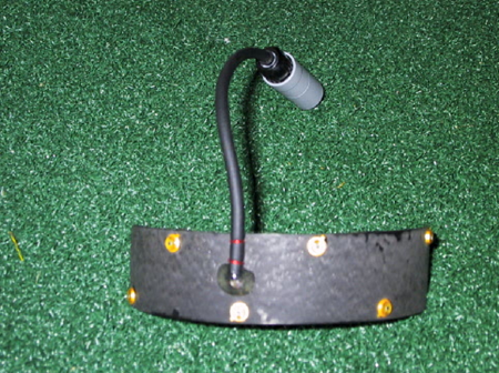
Scapular kinematics have not often been measured in pitching biomechanics studies primarily because of limitations in equipment and techniques. There can be large skin motion artifacts at the scapula due to soft tissue effects, and in order to measure the 3 DOF scapular rotations, at least 3 non-collinear markers are needed to define the scapula. Previously, limitations in camera resolution prevented measurement of three reflective markers placed over a relatively small area of the acromion, where there is less skin motion. Magnetic tracking systems have also been used for analyzing scapular kinematics, however these clinical studies have analyzed slow and constrained movements, and the sampling frequencies (up to 150 Hz) are too slow for measuring the acceleration phase of the pitching motion. Additionally, the use of wired sensors may preclude their use in high-speed motion actions as the cables have to be routed such that they don’t whip around during the violent acceleration phase of the pitching motion.
Chu 2012 took the Aguinaldo et al., 2007 study one step further in his dissertation as he measured 3 DOF for both scapular and humeral angular kinematics. Chu was very familiar with the ASMI methodology having published a paper with them in 2009 entitled Biomechanical Comparison Between Elite Female and Male Baseball Pitchers. The first study of scapular kinematics during baseball pitching was performed by Miyashita et al., 2010, but they only measured anterior/posterior tilt of the scapula in their study. Chu 2012 was the first to measure 3 DOF scapular rotations for the pitching motion using an optical motion capture system.
The GH head places greater stress on the anterior and inferior ligamentous structures with increased humeral external rotation. One of the goals of Chu’s study was to measure the contribution of both GH external rotation and anterior/posterior scapular tilt to the resultant shoulder external rotation angle that has been reported in other pitching biomechanics studies. Chu theorized that while different pitchers may both show the same magnitude of external rotation (e.g. 170°) using ASMI methodologies, they may not have the same risk of shoulder injury if one has 150° of GH external rotation and 20° of scapula posterior tilt, while the other has a 140°:30° relationship.
Chu used 28 reflective markers attached to anatomical landmarks on the subject’s body for his marker protocol. He used 5 arm markers for each arm, including two markers at the distal humerus at the lateral and medial malleoli, which allowed for direct measurement of 3 humeral rotational DOF. They also used two scapular triads that were attached to the flat portion of each shoulder’s acromion. With a marker at the tip of the acromion as well, they had 4 markers dedicated to measuring scapular kinematics. During a static trial, they also placed reference markers on scapular anatomical landmarks including the acromion angle (AA), TS, and AI. These reference markers were removed for the pitching trials. This methodology allowed them to directly measure 3 rotational DOF for both the scapula and the humerus. Details for the rest of the marker set can be found in Table 2 below.

Table 2: Anatomical Landmarks for Reflective Marker Placement (Table 4 in Chu 2012)
The methods used by Chu 2012 for the scapula and humerus segments are similar to the marker clustering technique used by Jackson et al., 2012. The technical markers, consisting of the scapula triad and the tip of acromion for each side, were used to capture scapular kinematics during the pitching trials. Knowing the rigid body relationship between the technical markers and the anatomical reference markers from the static trial, virtual reference markers were calculated for each time frame based on the measured 3D positions of the technical markers. This assumes that the spatial relationships between the technical markers and the reference markers remains constant during all movements as is required by rigid body assumptions. Chu did not utilize a chain model with an extended Kalman filter as Jackson et al. did in their 2012 study though.
Another improvement in the Chu 2012 study from the Aguinaldo et al., 2007 methodology was the full implementation of the STC of the ISB recommendations as published in Wu et al., 2005. LCSs were created for the thorax, scapula, and humerus for each time frame during the dynamic trials as shown in the figure below. Chu was able to accomplish this because they used 4 markers each for the thorax and scapula segments and 3 for the humerus segment. The 4 thorax markers were placed at C7, T8, jugular notch (IJ), and xiphoid process (PX) according to the ISB recommendations. This provides an upper torso, or thorax segment, that can accurately measure trunk hyperextension, which ASMI methodologies cannot.
Per the ISB recommendations, the humeral angular kinematics were defined with the humerus LCS relative to the thorax LCS, as shown in the figure below. The Euler sequence of Y-X’-Y’’ was used and represents plane of humeral elevation, humeral elevation, and humeral external/internal rotation. The scapular angular kinematics were defined similarly with the scapula LCS relative to the thorax LCS. The Cardan sequence of Y-X’-Z’’ was used and represented scapular protraction (+) / retraction(-), medial (+) / lateral (-) rotation, and anterior (-) / posterior (+) tilt.

At SFC, Chu 2012 reported that the scapula was positioned at 0.9±14.4° protraction, 23.3±9.8° lateral rotation, and 8.1±13.4° posterior tilt, while the PAS humerus was positioned at 90.1±10.6° abduction, 24.5±14.3° horizontal abduction, and 51.2±27.0° external rotation. The values for humeral external rotation generally agreed with previous values of 55±29° for Fleisig et al., 1999 and 54±24° for Chu et al., 2009 reported at SFC, despite different measurement methodologies. However, the scapular kinematic contribution at SFC are very minimal as shown in the figure below.

At shoulder MER, Chu 2012 reported that the scapula was positioned at 11.3±13.4° protraction, 33.8±7.2° lateral rotation, and 18.0±14.1° posterior tilt, while the PAS humerus was positioned at 95.1±8.2° abduction, 16.3±9.3° horizontal adduction, and 142.7±12.5° external rotation. The values for MER were much lower in this study than in the values in Table 1. Most studies have reported MER values of 170-180°; however, those values were a combination of GH rotation, scapular posterior tilt, and trunk extension. Chu eliminated the contribution of trunk extension to shoulder external/internal rotational values with his measurement technique for the thorax described previously. .
Chu 2012 measured the shoulder external rotation angle as the rotation of the humerus relative to the thorax following the ISB convention. As such, Chu’s measurement of shoulder external rotation angle includes both GH rotation and scapular posterior tilt, but does not include trunk extension. Scapular kinematics were measured as the rotation of the scapula relative to the thorax. As such, both humeral and scapular segmental rotations were measured relative to the thorax. However, we cannot just subtract the differences between the two curves in Figure 11 above to get humeral rotations relative to scapular rotations. That is because they used segmental rotations of the scapula relative to the thorax, where a Y-X’-Z” Cardan sequence is used, and for the humerus relative to the thorax, where a Y-X’-Y” Euler sequence is used. Posterior scapular tilt is the last rotation in the YX’Z” sequence, and GH rotation is the last rotation in the YX’Y” sequence, and they will be numerically different as they are calculated about different axes. Nonetheless, we can get a qualitative result regarding the contribution of GH external rotation and scapular posterior tilt using this methodology.
While using the conventions of the ISB of the STC provides more insight into the contribution of GH external rotation, scapular posterior tilt, and trunk hyperextension to reported values of GH MER during the pitching motion, it still does not quantitatively separate the contributions of GH external rotation and scapular posterior tilt. In order to do that, a purely kinematic chain joint rotation methodology would be required where the rotation of the distal segment is measured with respect to the proximal segment. For the complex shoulder problem, that would require measuring the clavicle relative to the thorax at the sternoclavicular (SC) joint, the scapula relative to the clavicle at the acromioclavicular (AC) joint, and the humerus relative to the scapula at the GH joint. However, measuring 3D clavicle rotations with reflective markers are very difficult as there are only two palpable bony landmarks and getting axial rotation of the clavicle is thus extremely difficult. Nonetheless, optimization routines have been used to estimate rotations about the clavicular long axis (Van der Helm and Pronk, 1995).
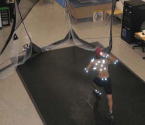
It should be noted that there were some limitations in the methodologies employed in this study that prevent direct comparison to other studies. Specifically, subjects did not pitch off of a mound to a catcher or target, rather they were instructed to throw maximal throws using a stride on flat ground into a net in front of them. Also, there was quite a range in the ability of the participants in this study and average velocities were lower than in previous pitching biomechanics studies. Nonetheless, direct comparison to other studies would not have been possible anyways as this study included a 3+ marker setup for each of the thorax, scapula, and PAS humerus segments. This allowed for direct measurement of 3 DOF segmental rotations for both the scapula and humerus relative to the thorax. This methodology eliminates trunk extension measurement from being included in the humeral external/internal rotation and angular velocity measurements. Thus, reported GH MER and internal rotational angular velocity values will be lower based on this methodological change, which more accurately captures the overhead throwing motion.
INERTIAL SENSOR – LAPINSKI (MIT)
Optical motion capture systems are good for generating three dimensional (3D) visualizations of a pitcher’s motion, but given the inherent limitations of ASMI methodologies, they do not provide a quantitatively accurate methodology for detailed biomechanical analysis of the overhead throwing motion. These systems directly record the instantaneous position of the tracked markers which inherently have noise in their measurements from the electronic camera system. Joint rotations, or angular kinematics, are calculated from the 3D positions of the markers using orthonormal vector calculations. From the estimated angular kinematics, angular velocities and accelerations are then calculated via numerical differentiation techniques. While these methodologies can provide reasonable estimates of 3D positions, every subsequent calculation may introduce mathematical inaccuracies in the data, which can be very problematic when estimating angular velocities of ultra high speed motions. Due to the inherent limitations and propagation of errors, optical motion tracking estimates of shoulder internal rotational angular velocity suffer from accuracy issues and can demonstrate large variance.
Berkson et al., 2006 first published an article entitled IMU Arrays: The Biomechanics of Baseball Pitching, that provided details on a proof-of-concept portable Inertial Measurement Unit (IMU) array developed at the MIT Media Lab that they later called SportSemble. This system was developed to provide direct measurements for acceleration and angular velocity in order to improve kinematic analysis of baseball pitching studies. They first used this system at the Boston Red Sox spring training in 2006 and results of the pilot study were reported in the Berkson et al., 2006 paper. Lapinski’s Masters Thesis entitled A Wearable, Wireless Sensor System for Sports Medicine was published in 2008 and provides details on the design of the system including technical specifications for the prototype SportSemble system. Lapinski tested 5 batters and 8 pitchers with a wireless 5 node system at the same Boston Red Sox spring training in 2006.
Lapinski et al., 2009 published a paper entitled A Distributed Wearable, Wireless Sensor System for Evaluating Professional Baseball Pitchers and Batters that reported the results for a second generation SportSemble system on 4 pitchers and 5 batters. The following figure was taken from Lapinski et al., 2009 (Figure 6) and shows the humeral internal rotational angular velocity measurements for two different pitchers.


Despite MLB pitching mechanics being relatively similar when comparing video of the pitchers’ humeral internal rotation during the arm acceleration phase, pitchers demonstrate unique angular velocity signatures when one examines appropriate metrics. The plots above show that despite general similarities in the curves for the different pitchers, there are definite differences between the two pitchers. Each pitcher demonstrated unique high-speed signatures describing their individual shoulder mechanics.

By recreating the signal and scaling it appropriately, I can overlay the 2 plots with appropriate time and angular velocity scales for the two plots to better demonstrate these differences. As one can see in the figure above, there are significant differences between the two players. Analysis of this type of data is what is needed to profile different pitching styles and to more importantly quantify injury potential. How the arm accelerates and decelerates is absolutely necessary for truly analyzing injury mechanics of the violent overhead throwing motion. Results like this from inertial sensors are the future of pitching performance analysis.
Table 3 shown below is taken from Lapinski et al., 2009 (Table 2 in their paper) and provides average peak shoulder internal rotational angular velocity values for 4 different pitchers comparing values for both the IMU array and calculations from an optical motion capture system. Notice that there are differences between the two systems. If done appropriately and the motion capture data internal rotation angular velocity rates are specified in the appropriate humeral longitudinal axis, then the values should be nearly the same (see this link for details on how to perform this), except for some potential misalignment in coordinate axes and/or inertial sensor movement. That is a big problem with using motion capture angular velocity rates, as they can vary from study to study. One commonality is that the variance from optical motion capture studies for shoulder internal rotation angular velocity values will be much higher as the magnitudes during the motion will change with the order of rotations for each pitch. Whereas the angular velocity rates aligned with the longitudinal humeral axis will strictly be a function of the true variance in the magnitude of this value, with some potential noise due to sensor movement. The average standard deviation of the IMU array was about 6% whereas the average standard deviation of the optical system was 15%.

Table 3: (Taken from Table 2 in Lapinski et al., 2009)
Lapinski 2013 presented more inertial sensor data outputs from both pitching and hitting sessions in his MIT dissertation. As before, the MIT group tested their node platform with players from the Boston Red Sox. This paper provides more background on the inertial sensor system itself, however there are some very interesting data outputs in there. Specifically, comparisons of dual system kinematic outputs for pitching biomechanics highlight many of the deficiencies with optical motion capture systems.
While providing a dual system comparison is an excellent methodology for comparing the two systems, it is somewhat limited as no methodology is provided for how they calculated optical camera-based kinematic outputs. Data is presented as though it is measured in the same global axes, however there is no discussion of methodology to support this. Unfortunately, I cannot speak to the accuracy of the optical kinematic calculations as no methodologies were presented for this.
Nonetheless, this paper provides some very good outputs showing differences between the two systems. The first figure below taken from Lapinski 2013 is a general example showing the General Stat Sheet output they provide, which shows values for different pitches as well as curves for all of the sensor data. Closer examination shows large differences in angular velocity measurements for different pitch types.

The next plot is an adaptation of the 6 phases of the pitching motion often presented in the ASMI studies color coded to the PAS angular velocity output from the inertial sensor. A couple of interesting things. First, the magnitude of humeral angular velocity is just above 4,000 deg/sec. This again is much lower than the typical optical camera based values presented earlier. Second, one can see more fidelity in the gyroscope data during arm cocking and acceleration phases that is typically missing in optical data due to filtering effects.


The increased fidelity in the inertial sensor measurements is extremely valuable and necessary for analyzing UCL injury risk that is just not possible with optical kinematic outputs. Below is a graph taken from Lapinski 2013 which plots both shoulder angular velocity and shoulder angular acceleration. From this graph we can see that the rate of shoulder acceleration (green line) peaks just before the peak value for shoulder angular velocity (blue line) and then undergoes a significant deceleration in only 20 milliseconds (Note: I believe there are some false readings near peak deceleration due to combined effects of centripetal acceleration on angular velocity sensor measurement and the actual ball release which tends to cause spikes in acceleration curves). Nonetheless, this shows how much angular acceleration can change in a very short time frame. This is critical information as it is directly related to joint torques, which has a direct effect on UCL loading rates. Optical data outputs cannot provide this type of fidelity in calculated accelerations due to filtering of the positional data.

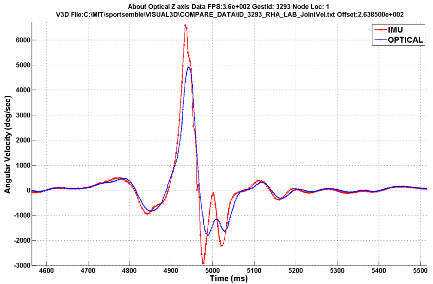
The figure below was taken from Lapinski 2013 and shows a comparison of angular velocity data for the Z axis of the hand for both IMU and optical data. As discussed previously, I cannot verify that these calculations are referencing measurements in the same coordinate system using a local (body) angular rate to Euler rate transformation. If we assume data is presented properly in the same coordinate systems (as the plots say about the optical Z axis), then we can clearly see differences between the two systems. This figure shows that the optical data is clearly attenuated relative to the IMU data, which is expected when 3D positional data is filtered to produce smooth velocity and accelerations.

The following figure shows the same plot but without filtering of the optical data. One can see that by not filtering the data, the optical data better matches the IMU data but still is lower in peak magnitude, but it also has high frequency electrical noise from the camera system along the waveform.
 Another problem with filtering of optical data is the effect that it has on the fidelity of the signal. By definition of 3D positional data filtering, the resultant velocities and accelerations will be smoothed curves, which eliminates some of the IMU content that is important for accelerations and decelerations. The figure below shows a comparison between the 2 systems for shoulder angular velocity data about the optical Y axis. While the optical data tracks fairly well, it obviously is missing the fidelity of the IMU system.
 This can be more clearly seen when we differentiate the angular velocity signal to get the angular acceleration signal. The green signal is the IMU angular acceleration and the blue is the optical angular acceleration. There is clearly a difference between the two systems. The red signal is the same green signal but downsampled to 360 Hz to mimic the sampling rate of the optical system. This shows the influence of sampling rate on angular acceleration data as well.

Lapinski 2013 provides some very compelling details on the use of an inertial node system for kinetic analysis of pitching biomechanics. That is beyond the scope of this article and will be presented in a subsequent post. Nonetheless, Lapinski shows how inertial sensor outputs can be combined with optical positional and orientation outputs in a hybrid optical-inertial data model and used as input data for subsequent kinetic analysis. This technique essentially combines the benefits of both systems and can be a very powerful tool for creating more accurate and realistic bio-dynamic simulation models.
SUMMARY
Given the importance of the extremely complex shoulder girdle in the overhead throwing motion, appropriate measurement systems are necessary in order to provide quantitative performance and injury risk analysis. No other joint demands the combination of extreme mobility and dynamic stability as the pitching arm shoulder. To date, most pitching biomechanics studies have been performed with optical motion capture systems which provide adequate visualizations, but often suffer from accuracy and large variance issues, especially when used as inputs to modern physics-based simulation models.
Inertial sensor technologies are becoming more common in high-speed sports science applications. These technologies provide direct measurement of translational accelerations and angular velocities with higher sampling frequencies and real-time capabilities. Results from these systems can be used to more directly infer joint loads and torques, as well as estimate the effects of fatigue with the use of intelligent algorithms. It is important that sports scientists understand the differences in angular velocity measurements between optical motion capture and inertial sensor systems.
More importantly, a critical review of optical camera and inertial sensor based studies of pitching biomechanics has shown that sports scientists have to be careful when comparing results from the two measurement systems. There are methodologies for getting direct comparisons, but most scientists do not use this important step. Additionally, optical camera systems provide kinematic data in the velocity and acceleration domains that are often attenuated and missing critical acceleration and deceleration components due to filtering effects.
This will have a direct effect on any player profiling studies, determining angular accelerations, and as inputs to any forward dynamics simulations. All 3 of these advanced scientific studies are absolutely necessary to advance the study of pitching biomechanics from qualitative research studies to scientific studies capable of quantifying both performance differences and injury probabilities. As the necessary measurement systems are finally becoming more commercially available, the next step is for sports scientists to integrate inertial sensor systems into these advanced biomechanical studies to significantly advance baseball research.
APPENDIX A: ARM KINEMATIC METHODOLOGY IMPROVEMENTS
As was discussed in detail on the ASMI limitations page, I personally would not use only 2 markers on the PAS humerus, as was done in both the ASMI and SDCHP studies. It leaves too much potential inherent error in the humeral kinematic gauge R&R which immediately challenges the validity of the kinematic outputs. There are too many alternatives that will provide more accurate measurements than using a technique that was initially implemented over 20 years ago due to limitations in camera technology at the time. There are 2 specific techniques that can be applied to problematic studies like this: 1.) marker clusters of more than 3 markers per body segment, and 2.) advanced algorithms to reduce noise in motion data using a kinematic chain model with an extended Kalman filter.
Using more than 3 non-collinear markers per body segment allows for measurement of up to 3 rotational DOF. The additional markers provide redundant 3D positional data that can be used to provide a better estimate of the underlying segmental orientation (Cappello et al., 1997). Least-squares optimization routines are typically used with the time series positional data for all of the markers in the cluster to define a rigid body orientation for the body segment. Even if a marker(s) is out of view for one frame, the other markers can still be used to estimate the rigid body pose, assuming that at least 3 non-collinear markers are simultaneously in view for each frame.
Jackson et al., 2012 provide details on implementing both marker clusters and an extended Kalman filter in their paper Improvements in measuring shoulder joint kinematics. They used a combination of anatomical markers, which were placed on bony landmarks, and technical markers, that were located in areas that minimized marker movement relative to the underlying bone during muscle contractions (Cappozzo et al., 2005). The anatomical markers were only used for calibrating joint centers relative to anatomical landmarks. The technical markers were used in a clustering technique to define the segmental motion based on redundant marker sets. Jackson et al., 2012 also imposed constraints on the motion of the joints through a kinematic chain model with an extended Kalman filter to reduce the noise on the markers in the cluster. This is a much more accurate alternative for measuring 3 DOF of the humeral segment directly.
Any time you only use 2 markers on the humerus to measure 3 DOF at the shoulder joint, you open yourself up to questionable data outputs given the gauge R&R problems discussed previously. If it is that big of a problem to use at least 3 markers on the humerus with a particular optical motion tracking system, then that measurement system is most likely not the right solution for a problem as demanding as the overhead throwing motion of professional baseball players.
In the Golf Sports Science Research page, I detailed some of the methodologies that I implemented in the Callaway Golf Player Performance Bay. Not unlike ASMI or SDCHP, I had to make choices in regards to measurement systems, marker protocols, and kinematic algorithms. However, our motion capture data was not just being analyzed for kinematic analysis. Rather, motion data outputs were interfacing with a variety of synergistic R&D projects which meant that accuracy of the calculated kinematic data output was paramount as it was being used as an input to a secondary study. If the measurement methodologies we employed did not meet the scrutiny of gauge R&R studies, then we had to search for better alternatives. Because we had strict requirements for the kinematic output data as it was used as inputs for player profiling, simulation, and modeling programs, that meant constant testing and validation of our underlying measurement systems to verify that rigid body outputs for each body segment provided accurate and repeatable kinematic output data.

Based on our system testing, we employed a measurement protocol that used curved composite plates with more than 3+ markers for each segment in a marker clustering setup, a vector-based kinematic chain algorithm where each joint’s rotational DOF were measured relative to the more proximal segment (with the pelvis 6 DOF motion measured relative to the lab coordinate system), and an extended Kalman filtering algorithm that minimized optoelectronic marker noise and occlusions with the kinematic chain model to more accurately predict body segment rotations relative to the proximal segment. This was all done with some marker cluster plates that had to be attached over clothing which was required for use in the Player Performance Bay. The combination of these techniques provided more accurate body segment orientation data than using a typical anatomical marker protocol.
While that particular setup would not work with the more extreme mobility of the PAS extremity in ultra high-speed overhead throwing mechanics, the point is that the sports scientist has to find a methodology that provides the most accurate data possible that best represents the underlying skeletal motion. In pitching biomechanics, humeral rotations are absolutely critical for both performance and injury analysis as the humerus interfaces proximally at the GH joint and distally at the elbow joint. The musculotendon tissues, ligaments, and the proximal and distal humeral surfaces that they connect to are what gets damaged in elite pitchers during the violent overhead throwing motion. Implementing a measurement system and methodology that does not accurately measure the 3 DOF rotations of this critical body segment severely limits the potential quantitative performance and injury analysis capabilities of the output data. How can a detailed study on UCL injuries ever be performed if we only have approximate humeral rotational data available? Twenty years ago this may have been a reality; that no longer has to be the case. A combination of an appropriate measurement system, marker protocol, and/or intelligent algorithm can be found to provide optimal solutions for any advanced biomechanical high-speed motion study.