The following demonstrates the fundamental skills necessary for managing rigid body reference frames and the kinematics of vectors. It is essential that this material be mastered, not simply understood, in order to carry out two and three dimensional analyses of biomechanical problems. This information is taken directly from Dr. Gary Yamaguchi’s outstanding book Dynamic Modeling of Musculoskeletal Motion.
DIRECTION COSINES
Direction cosines define angular relationships between bases. The figure below shows a planar movement of the lower leg with respect to the ground during level walking. The ground segment (N) presents a horizontal surface, with n1 pointing in the direction of travel and n2 pointing vertically upward. The “plane of motion” is defined by basis vectors n1 and n2. Reference frame A defines the orientations of the shank with respect to N. Angle q1 describes the magnitude of angular rotation between A and N in the plane of motion.  The relationship between the N basis vectors and the A basis vectors are derived via vector addition. As shown in, B, the a1 vector can be decomposed into composite horizontal and vertical components. Since all of the individual basis vectors have lengths equal to 1, the horizontal component of a1 has magnitude (1) cos (q1) and points in the +n1 direction. The vertical component has magnitude (1) sin (q1) and direction +n2. Thus,
 ![]() Similarly, a2 can be constructed from composite vectors in the –n1 and +n2 directions (C).
Similarly, a2 can be constructed from composite vectors in the –n1 and +n2 directions (C). ![]() The basis vector a3 remains parallel to n3, and thus is equivalent.
The basis vector a3 remains parallel to n3, and thus is equivalent. ![]() Organizing these into a table with the “fixed” (or more proximal) reference frame on the left and the “moving” (or more distal) reference frame above and to the right,
Organizing these into a table with the “fixed” (or more proximal) reference frame on the left and the “moving” (or more distal) reference frame above and to the right,  This table, which defines the n1, n2, and n3 components of vectors a1, a2, and a3 (and the a1, a2, and a3 components of vectors n1, n2, and n3) is referred to as a table of direction cosines. The direction cosines themselves are the elements of the table – and include the sines and numerals too. To save writing, cos(q1) and sin(q1) are abbreviated c1 and s1,
 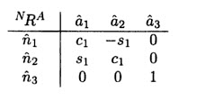 It is clear from this construction that there is only one degree of freedom relating the N and A bases (angle q1). This table is typical of a simple rotation about the common a3 and n3 axis. A simple rotation is one in which the direction (but not necessarily the location) of the axis of revolution between frames remains fixed. Here, no matter how much A is rotated from N by angle q1, a3 and n3 remain fixed in orientation and parallel to each other, and hence the rotation is classified as a simple rotation. Direction cosines from simple rotations about a common basis vector always have two cosines aligned diagonally, one positive and one negative sine aligned along the other diagonal , and one row and one column each with 2 zeros and a one. The one shows that the axis of the rotation is fixed in direction and parallel to both the a3 and n3 directions.
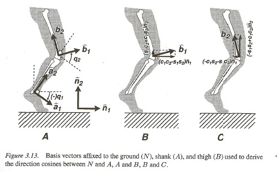
DIRECTION COSINES IN PLANAR MOTIONS
Now we can also include a rotation at the knee as well as the previous rotation at the ankle. If rigid body B (thigh) rotates by angle q2 from rigid body A (shank or lower leg), and A rotates from N as defined previously, then additional direction cosines may be defined. The figure above shows this case where the motions of the femur (B) and the shank (A) are coplanar. The following direction cosine tables now describe the simple rotation from N to A, and the simple rotation from A to B,  A compound rotation from N to B can easily be defined via substitution:
 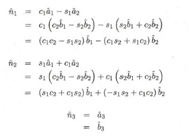 Therefore, the table defining the direction cosines between the N and the B bases can be expressed as:
 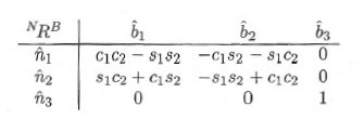 This logic can easily be extended to systems having many more planar degrees of freedom.
DIRECTION COSINES IN 3D
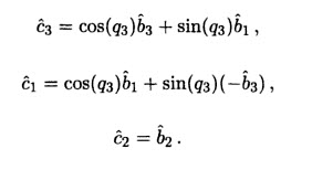
The direction cosines.for any sequence of simple rotations can be performed in exactly the same way as the above examples. Using the direction cosine tables for each simple rotation, the relationships between basis vectors can be defined for a noncoplanar compound rotation. For example, let’s introduce a third simple rotation by angle q3 is defined about the b2 axis in the example above, bringing into existence a fourth reference frame C. Anatomically, angle q3 corresponds to a rotation of the pelvis about the axis of the femoral shaft.

The direction cosines from B to C are derived by first drawing the two sets of basis vectors in such a way that the viewing direction is parallel to the rotation axis. In other words, the drawing of the basis vectors depicts the rotation axis (in this case, b2 and c2) as pointing perpendicularly into or out of the drawing. One should also check if right-handed reference frames and bases are used and consistent througout, and if each drawing made from a different viewpoint correctly reflects the right-handed nature of the coordinate frames. In other words, that the “1” axis crossed by the “2” axis yields the “3” axis. An arc defining the the angle of positive rotations is also drawn to complete the diagram.
Typically the two bases are defined so they are coincident when the rotation angle is zero. One basis can be thought of as being “fixed” (usually drawn with the horizontal and vertical axes), and the other basis as “rotating”. For the purpose of defining direction cosines only, the user will find it less confusing to always redraw the rotated basis with the rotation angle positive and less than 90 degrees.
Next, the direction cosines are derived by selecting one of the “rotating” vectors at a time, and decomposing them into a vector sum of “fixed” vectors multiplied by the appropriate sines or cosines. For this example,
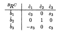
 With the “fixed” frame on the left, and the “rotating” frame listed above and to the right, the simple rotation can be represented by:
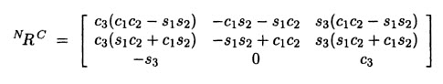
 If the direction cosines relating the N frame to the C frame are desired, they can be found via substitution using shorthand notation for sine and cosine and the tables listed the previous 2 figures:

From these equations, the entries in the direction cosine table can be made:
 ROTATION MATRICES
Matrix multiplication is an alternative to using tedious substitution in finding the table of direction cosines from N to C. First, the nine entries in each table of direction cosines are written in matrix form; that is in the same row-column order but without the basis vectors. The previous table above written in matrix form would be:
NRC is called “the rotation matrix from N to C”, with the superscripts being read from left to right. Note that the left superscript corresponds to the basis indicated by the basis vectors written on the left-hand side of the direction cosine table, and the right superscript corresponds to the basis indicated by the basis vectors written above and on the right hand side of the direction cosine table. As another example, the rotation matrices from N to B and B to C from the previous examples can be expressed as below:

In matrix multiplication form,
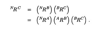 The interior subscripts A and B can be thought of as “cancelling each other” when they appear as adjacent right and left superscripts, leaving only the exterior superscripts N on the left and C on the right. The order of the matrix multiplication is important, and the cancellation method serves as a safeguard against performing a matrix multiplication in the wrong order.
PROPERTIES OF ROTATION MATRICES
Rotation matrices relating one set of basis vectors to another are 3 x 3 examples of orthonormal matrices. Orthonormal matrices have several important properties which can be exploited to simplify kinematic and dynamic biomechanical analyses.
By definition, orthonormal matrices have rows and columns containing the measure numbers of unit vectors. Hence, it is almost trivial to state that each row and column has a vector magnitude of exactly 1. It is less apparent when looking at the product of several matrix multiplications that the sum of the squares of each row and column is 1. By definition, the row elements of orthonormal matrices form vectors perpendicular to each other, and the column elements of orthonormal matrices form vectors perpendicular to each other.
EULER ANGLES AND OTHER ROTATION SETS
The famous mathematician Euler recognized that a series of three rotations could be used to uniquely define the orientation of a rigid body in 3D space. Though there are many sets of three sequential rotations which lead to a unique orientation of a rigid body, the most commonly used are Euler rotations.
The figure above shows a series of rotations of the pelvis relative to the fixed femur. Initially, the pelvis reference frame P is considered to be coincident with the right femoral reference frame F, oriented such that f3 points anteriorly, f1 points laterally, and f2 points inferiorly. This orientation is chosen because the resulting Euler rotations form a 3-1′-3” set (a z-x’-z” sequence in Cartesian space), meaning that the first rotation occurs about the “3” axis, the second rotation occurs about the once rotated “1” axis, and the third rotation occurs about the twice rotated “3” axis. Each rotation is a simple rotation, and brings the P frame to an intermediate orientation. In the final orientation picture above (B) shows the pelvis in its final orientation after three successive rotations have been performed:
- Rotation about common f3, p3’ axis. From the initial orientation that is coincident with the F frame, the first intermediate orientation P’ is achieved by a simple rotation about the common f3, p3’ axis (C). Figure C above shows the first two basis vectors of F and P’ superimposed. It should be understood that the f3 and p3’ axes are colinear, and point perpendicularly out of the paper. Angle q1 is defined positively when the rotation of p1’ is counterclockwise from f1, consistent with the angular representation for the f3, p3’ axis. The view is defined with the f3, p3’ unit vectors pointing out of the paper (directly at the viewer), and with the angle q1 positive and less than 90 degrees.
 A negative rotation corresponds to pelvic list (drooping of the pelvis to the left in the frontal plane) or hip adduction. Hip abduction occurs with a positive rotation angle.
 - Rotation about the common p1’, p1’’ axis. The next intermediate orientation P’’ is obtained by a second simple rotation about the common p1’, p1’’ axis (D). A drawing of the basis vectors looking directly at the common p1’, p1’’ axis is made as an aid to the derivation of the table elements.
 When q1 is small, a positive value of the rotation angle q2 approximates hip extension. In the unusual event that q1 is large, it would be incorrect to refer to q2 as the hip extension angle. This is because hip extension is usually defined in the vertical sagittal plane, and if the hip is abducted or adducted the rotation axis p1’, which is perpendicular to the p2’, p3’ plane, will not be perpendicular to the vertical sagittal plane.
 - Rotation about the common p3’’, p3 axis. The final rotation (E) leads to the orientation of the pelvis P.


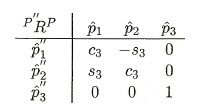
The table of direction cosines relating the femoral (F) and pelvic (P) reference frames is obtained most simply via matrix multiplication, which yields the rotation matrix FRP and its corresponding table of direction cosines,
 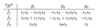 Direction cosines for virtually any compound rotation can be found easily by using this exact methodology. One needs only to define the sequence of simple rotations comprising the compound rotations, and to perform the matrix multiplications correctly.